728x90

잘 정제된 음성 데이터셋의 경우 (특히 딥러닝 음성인식 및 오디오 처리 학습용의 경우) 거의 Mono channel로 공개가 되어있다.


하지만 다양한 실환경에서 녹음된 오디오 데이터셋의 경우, 녹음 기기에 따라 2이상의 channel로 구성된, Stereo channel로 공개가 된 데이터들이 많다.


간단하게 아래와 같이 음성을 로드하게 되면

import torchaudio
import torch

waveform = './test.wav'
y, sr = torchaudio.load(waveform)


y의 size를 출력해보면, 예를 들어, (2, 100) 과 같이 나올 수가 있다.


이를 Stereo channel이라고 한다.


간단하게 아래의 그림을 보면 이해가 쉽게 될 것 같은데, stereo는 채널 별 들리는 소리가 약간 다른 반면, mono는 stereo의 평균을 낸 것으로 간주할 수 있다.

https://soundskrit.ca/2023/06/26/stereo-sound-vs-mono-explained/


우리가 해결하고자 하는건, 어쨋든 n-channel 이상의 waveform에 대해 평균을 내주어 mono channel로 만드는 것으로 간주할 수 있다. 


아래와 같이 해결하면 된다.


import torchaudio
import torch

waveform = './test.wav'
y, sr = torchaudio.load(waveform)
waveform_mono = torch.mean(y, dim=0).unsqueeze(0)


위와 같이 진행하면 waveform_mono는 (1, 100)의 형태로 얻어질 수 있다.

728x90
728x90

LibriSpeech, Libri-Light, Multilingual LibriSpeech (MLS) 등...


나 같은 경우는 윈도우에서 다운받아서 그것을 작업 서버로 옮겨야하는,


굉장히 비효율적인 그런 행동을 자주 하곤 했다.


국내 AIHUB 데이터셋은 이런식으로 다운받아야해서 얼마나 짜증나는지 모르겠다. 


게다가 연구실에 대용량 데이터셋 다운받게 되면 전체적으로 인터넷도 느려지고,


MobaXterm으로 옮기다 보면 도중에 죽는 경우도 많아서 정말 짜증나는 일이다.


오늘 예시로 해볼것은 우분투에서 wget을 사용하여 LibriSpeech (http://www.openslr.org/12) 의 dev-clean.tar.gz 을 다운받아보겠다.


아래는 해당 사이트 그림인데


여기에서 왼쪽 최하단의 부분을 보면 주소가 제공된다.


https://www.openslr.org/resources/12/dev-clean.tar.gz 


그다음 wget https://www.openslr.org/resources/12/dev-clean.tar.gz 하면 끝난다


우분투 내 실행화면은 아래와 같다


음 정말 간단하다


이렇게 하면 3TB 짜리 Libri-Light 받는 것도 부담 없겠다.


AIHUB 데이터셋은 특정 프로그램을 이용해서 다운받아야 되는데 정말 짜증나는 일이다. 


얼른 고쳐주면 좋겠다.

728x90
728x90

음성 인식 테스크에서 pcm 파일을 direct로 읽어야 할 때가 있는데, 이 때 두 가지의 코드를 주로 사용한다.


오늘은 이에 대해 생각 정리 겸 실험 내용을 저장하기 위해 작성한다.


1. numpy memmap으로 읽을 경우


이 때에는, 읽은 pcm 파일을 그대로 저장하게 되면 음성의 magnitude가 굉장히 크기 때문에 max value인 32767로 나눠주어야 한다.


signal = np.memmap(sample_data, dtype='h', mode='r').astype('float32')

signal = signal / 32767


2. numpy frombuffer + librosa로 읽을 경우


1번과는 다르게 따로 나눠줄 필요는 없다.


with open(sample_data, 'rb') as opened_pcm_file:
    buf = opened_pcm_file.read()
    pcm_data = np.frombuffer(buf, dtype = 'int16')
    wav_data = librosa.util.buf_to_float(pcm_data, 2)


3. 음질 결과 비교 


1번:

method1_16000.wav
0.07MB


2번: 

method2_16000.wav
0.07MB


1번의 32767로 normalized 한 파일과 2번 방식으로 읽은 파일은 서로 데이터의 크기가 같다.


4. 변환 속도 비교

1번과 2번의 시간 비교는 아래와 같다.

2번이 약 2배 이상 빠른것을 알 수 있다.


5. 결론

두 방법 모두 가능하지만, 대규모 데이터셋을 처리하기 위해서는 2번 방법을 사용하는 것이 좋을 것 같다.


예를 들어 KoSpeech 같은 경우 각 음성 파일의 길이 비교 없이 training set 62만개에 대해서 10에폭을 돌린다고 하면


1번 방법: 620,000 * 10 * 0.00054 = 3,348 = 0.93시간

2번 방법: 620,000 * 10 * 0.00026 = 1,612 = 0.44시간


의 차이가 data loading 할 때 발생한다.


전체 코드


import soundfile as sf
import os
import numpy as np
import time

sample_data = './45.pcm'
data_dir = './check_pcm/'

start = time.time()
signal = np.memmap(sample_data, dtype='h', mode='r').astype('float32')
print(signal.shape)

signal = signal / 32767
print('method1 takes {}'.format(time.time() - start))


sf.write(os.path.join(data_dir, 'method1_16000.wav'), signal, 16000, format='WAV', endian='LITTLE', subtype='PCM_16')

import librosa
start = time.time()
with open(sample_data, 'rb') as opened_pcm_file:
    buf = opened_pcm_file.read()
    pcm_data = np.frombuffer(buf, dtype = 'int16')
    wav_data = librosa.util.buf_to_float(pcm_data, 2)
print('method2 takes {}'.format(time.time() - start))    

sf.write(os.path.join(data_dir, 'method2_16000.wav'), wav_data, 16000, format='WAV', endian='LITTLE', subtype='PCM_16')


pcm 파일의 sampling rate는 어떻게 구할 수 있을까? 다음번에는 이 문제와 관련된 issue 정리해보기

728x90
728x90

이번에는 RNN을 MNIST로 돌려보는 것을 코딩해본다.


Experimental setups

import torch
import torch.nn as nn
import torch.nn.functional as F
import torch.optim as optim
from torchvision import datasets, transforms
from torch.autograd import Variable
import os
import matplotlib.pyplot as plt
import numpy as np
torch.__version__

device = torch.device('cuda' if torch.cuda.is_available() else 'cpu')
torch.manual_seed(2891)
num_gpu = 1
if torch.cuda.device_count() > 1:
    num_gpu = torch.cuda.device_count()
print("Let's use", num_gpu, "GPUs!")
print('our device', device)

'''
Let's use 1 GPUs!
our device cuda
'''


RNN 모델 설계

class RNN(nn.Module):
    def __init__(self, input_size, hidden_size, num_layers, num_classes):
        super(RNN, self).__init__()
        
        self.hidden_size = hidden_size
        self.num_layers = num_layers
        self.lstm = nn.LSTM(input_size, self.hidden_size, self.num_layers, batch_first=True)
        self.gru = nn.GRU(input_size, self.hidden_size, self.num_layers, batch_first=True)
        self.fc = nn.Linear(self.hidden_size, num_classes)
        
        
    def forward(self, x, rnn):
        
        if rnn == 'lstm':
            rnn_layer = self.lstm
            h0 = torch.zeros(self.num_layers, x.size(0), self.hidden_size).to(device) 
            c0 = torch.zeros(self.num_layers, x.size(0), self.hidden_size).to(device)
            out, _ = self.lstm(x, (h0, c0))
        else:
            rnn_layer = self.gru
            h = torch.zeros(self.num_layers, x.size(0), self.hidden_size).to(device) 
            out, _ = self.gru(x, h)
        
        out = self.fc(out[:, -1, :])
        return out

model call시 원하는 rnn 계열 (lstm, gru) 선택 가능하도록 구현함


Parameter & Model shape & Hyper-parameter check 

sequence_length = 28
input_size = 28
hidden_size = 128
num_layers = 2
num_classes = 10
batch_size = 100
num_epochs = 10
learning_rate = 0.01

model = RNN(input_size, hidden_size, num_layers, num_classes).to(device)
#model shape
for p in model.parameters():
    print(p.size())
'''
torch.Size([512, 28])
torch.Size([512, 128])
torch.Size([512])
torch.Size([512])
torch.Size([512, 128])
torch.Size([512])
torch.Size([512])
torch.Size([384, 28])
torch.Size([384, 128])
torch.Size([384])
torch.Size([384])
torch.Size([384, 128])
torch.Size([384])
torch.Size([384])
torch.Size([10, 128])
torch.Size([10])
'''
def count_parameters(model):
    return sum(p.numel() for p in model.parameters() if p.requires_grad)

model_hp = count_parameters(model)
print('model"s hyper parameters', model_hp)
# model"s hyper parameters 374026


Dataset load, train, test loader 선언

train_loader = torch.utils.data.DataLoader(datasets.MNIST('data', train=True, download=True, transform=transforms.ToTensor()),batch_size=batch_size, shuffle=True)
print(len(train_loader)) # 600
test_loader = torch.utils.data.DataLoader(datasets.MNIST('data', train=False, transform=transforms.ToTensor()),batch_size=1000)
print(len(test_loader)) # 10
'''
Downloading http://yann.lecun.com/exdb/mnist/train-images-idx3-ubyte.gz
Downloading http://yann.lecun.com/exdb/mnist/train-images-idx3-ubyte.gz to data/MNIST/raw/train-images-idx3-ubyte.gz
9913344/? [04:53<00:00, 33768.69it/s]

Extracting data/MNIST/raw/train-images-idx3-ubyte.gz to data/MNIST/raw

Downloading http://yann.lecun.com/exdb/mnist/train-labels-idx1-ubyte.gz
Downloading http://yann.lecun.com/exdb/mnist/train-labels-idx1-ubyte.gz to data/MNIST/raw/train-labels-idx1-ubyte.gz
29696/? [00:00<00:00, 433940.88it/s]

Extracting data/MNIST/raw/train-labels-idx1-ubyte.gz to data/MNIST/raw

Downloading http://yann.lecun.com/exdb/mnist/t10k-images-idx3-ubyte.gz
Downloading http://yann.lecun.com/exdb/mnist/t10k-images-idx3-ubyte.gz to data/MNIST/raw/t10k-images-idx3-ubyte.gz
1649664/? [00:51<00:00, 32232.92it/s]

Extracting data/MNIST/raw/t10k-images-idx3-ubyte.gz to data/MNIST/raw

Downloading http://yann.lecun.com/exdb/mnist/t10k-labels-idx1-ubyte.gz
Downloading http://yann.lecun.com/exdb/mnist/t10k-labels-idx1-ubyte.gz to data/MNIST/raw/t10k-labels-idx1-ubyte.gz
5120/? [00:00<00:00, 108088.65it/s]

Extracting data/MNIST/raw/t10k-labels-idx1-ubyte.gz to data/MNIST/raw

Processing...
Done!
600
10
/usr/local/lib/python3.7/dist-packages/torchvision/datasets/mnist.py:502: UserWarning: The given NumPy array is not writeable, and PyTorch does not support non-writeable tensors. This means you can write to the underlying (supposedly non-writeable) NumPy array using the tensor. You may want to copy the array to protect its data or make it writeable before converting it to a tensor. This type of warning will be suppressed for the rest of this program. (Triggered internally at  /pytorch/torch/csrc/utils/tensor_numpy.cpp:143.)
  return torch.from_numpy(parsed.astype(m[2], copy=False)).view(*s)
'''


Loss, optimizer 선언

이전에는 F.nll_loss로 하였는데, 이번에는 CrossEntropy loss를 선언하여 진행함

criterion = nn.CrossEntropyLoss()
optimizer = torch.optim.Adam(model.parameters(), lr=learning_rate)


Training 진행

model.train()
total_loss = 0
total_acc = 0
train_loss = []
train_accuracy = []
i = 0
for epoch in range(num_epochs):
    for data, target in train_loader:
        data = data.reshape(-1, sequence_length, input_size).to(device)
        target = target.to(device)
         
        optimizer.zero_grad()
        output = model(data, 'lstm')
        loss = criterion(output, target)
       
        
        loss.backward()    # calc gradients
       
        total_loss += loss
       
        train_loss.append(total_loss/i)
        optimizer.step()   # update gradients
       
        prediction = output.data.max(1)[1]   # first column has actual prob.
        accuracy = prediction.eq(target.data).sum()/batch_size*100
       
        total_acc += accuracy
       
        train_accuracy.append(total_acc/i)
       
        if i % 10 == 0:
            print('Epoch: {}\t Train Step: {}\tLoss: {:.3f}\tAccuracy: {:.3f}'.format(epoch+1, i, loss, accuracy))
        i += 1
    print('Epoch: {} finished'.format(epoch+1))
'''
Epoch: 9 finished
Epoch: 10	 Train Step: 5400	Loss: 0.031	Accuracy: 99.000
Epoch: 10	 Train Step: 5410	Loss: 0.012	Accuracy: 100.000
Epoch: 10	 Train Step: 5420	Loss: 0.045	Accuracy: 99.000
Epoch: 10	 Train Step: 5430	Loss: 0.107	Accuracy: 98.000
Epoch: 10	 Train Step: 5440	Loss: 0.006	Accuracy: 100.000
Epoch: 10	 Train Step: 5450	Loss: 0.031	Accuracy: 99.000
Epoch: 10	 Train Step: 5460	Loss: 0.038	Accuracy: 98.000
Epoch: 10	 Train Step: 5470	Loss: 0.003	Accuracy: 100.000
Epoch: 10	 Train Step: 5480	Loss: 0.010	Accuracy: 100.000
Epoch: 10	 Train Step: 5490	Loss: 0.024	Accuracy: 100.000
Epoch: 10	 Train Step: 5500	Loss: 0.109	Accuracy: 97.000
Epoch: 10	 Train Step: 5510	Loss: 0.085	Accuracy: 96.000
Epoch: 10	 Train Step: 5520	Loss: 0.016	Accuracy: 100.000
Epoch: 10	 Train Step: 5530	Loss: 0.065	Accuracy: 99.000
Epoch: 10	 Train Step: 5540	Loss: 0.088	Accuracy: 98.000
Epoch: 10	 Train Step: 5550	Loss: 0.042	Accuracy: 99.000
Epoch: 10	 Train Step: 5560	Loss: 0.049	Accuracy: 98.000
Epoch: 10	 Train Step: 5570	Loss: 0.032	Accuracy: 99.000
Epoch: 10	 Train Step: 5580	Loss: 0.095	Accuracy: 97.000
Epoch: 10	 Train Step: 5590	Loss: 0.038	Accuracy: 98.000
Epoch: 10	 Train Step: 5600	Loss: 0.106	Accuracy: 98.000
Epoch: 10	 Train Step: 5610	Loss: 0.026	Accuracy: 99.000
Epoch: 10	 Train Step: 5620	Loss: 0.021	Accuracy: 100.000
Epoch: 10	 Train Step: 5630	Loss: 0.069	Accuracy: 98.000
Epoch: 10	 Train Step: 5640	Loss: 0.010	Accuracy: 100.000
Epoch: 10	 Train Step: 5650	Loss: 0.011	Accuracy: 100.000
Epoch: 10	 Train Step: 5660	Loss: 0.154	Accuracy: 97.000
Epoch: 10	 Train Step: 5670	Loss: 0.005	Accuracy: 100.000
Epoch: 10	 Train Step: 5680	Loss: 0.075	Accuracy: 97.000
Epoch: 10	 Train Step: 5690	Loss: 0.107	Accuracy: 97.000
Epoch: 10	 Train Step: 5700	Loss: 0.050	Accuracy: 98.000
Epoch: 10	 Train Step: 5710	Loss: 0.043	Accuracy: 98.000
Epoch: 10	 Train Step: 5720	Loss: 0.064	Accuracy: 99.000
Epoch: 10	 Train Step: 5730	Loss: 0.039	Accuracy: 98.000
Epoch: 10	 Train Step: 5740	Loss: 0.014	Accuracy: 100.000
Epoch: 10	 Train Step: 5750	Loss: 0.042	Accuracy: 99.000
Epoch: 10	 Train Step: 5760	Loss: 0.137	Accuracy: 96.000
Epoch: 10	 Train Step: 5770	Loss: 0.101	Accuracy: 97.000
Epoch: 10	 Train Step: 5780	Loss: 0.054	Accuracy: 97.000
Epoch: 10	 Train Step: 5790	Loss: 0.084	Accuracy: 97.000
Epoch: 10	 Train Step: 5800	Loss: 0.054	Accuracy: 98.000
Epoch: 10	 Train Step: 5810	Loss: 0.062	Accuracy: 97.000
Epoch: 10	 Train Step: 5820	Loss: 0.076	Accuracy: 98.000
Epoch: 10	 Train Step: 5830	Loss: 0.094	Accuracy: 97.000
Epoch: 10	 Train Step: 5840	Loss: 0.147	Accuracy: 96.000
Epoch: 10	 Train Step: 5850	Loss: 0.048	Accuracy: 99.000
Epoch: 10	 Train Step: 5860	Loss: 0.010	Accuracy: 100.000
Epoch: 10	 Train Step: 5870	Loss: 0.034	Accuracy: 98.000
Epoch: 10	 Train Step: 5880	Loss: 0.048	Accuracy: 99.000
Epoch: 10	 Train Step: 5890	Loss: 0.025	Accuracy: 99.000
Epoch: 10	 Train Step: 5900	Loss: 0.110	Accuracy: 97.000
Epoch: 10	 Train Step: 5910	Loss: 0.092	Accuracy: 98.000
Epoch: 10	 Train Step: 5920	Loss: 0.149	Accuracy: 96.000
Epoch: 10	 Train Step: 5930	Loss: 0.014	Accuracy: 100.000
Epoch: 10	 Train Step: 5940	Loss: 0.056	Accuracy: 98.000
Epoch: 10	 Train Step: 5950	Loss: 0.058	Accuracy: 97.000
Epoch: 10	 Train Step: 5960	Loss: 0.064	Accuracy: 98.000
Epoch: 10	 Train Step: 5970	Loss: 0.050	Accuracy: 98.000
Epoch: 10	 Train Step: 5980	Loss: 0.040	Accuracy: 99.000
Epoch: 10	 Train Step: 5990	Loss: 0.015	Accuracy: 100.000
Epoch: 10 finished
'''

RNN은 lstm으로 진행하였음


Plotting 결과

plt.figure()
plt.plot(np.arange(len(train_loss)), train_loss)
plt.show()
#plt.savefig('./train_loss_result.png')

plt.figure()
plt.plot(np.arange(len(train_accuracy)), train_accuracy)
plt.show()
#plt.savefig('./train_accuracy_result.png')


step에 따른 training loss 변화도
step에 따른 training accuracy 변화도


Evaluation 결과

with torch.no_grad():
    model.eval()
    correct = 0
   
    for data, target in test_loader:
        
        data = data.reshape(-1, sequence_length, input_size).to(device)
        target = target.to(device)        
        output = model(data, 'lstm')

        prediction = output.data.max(1)[1]
        correct += prediction.eq(target.data).sum()

print('\nTest set: Accuracy: {:.2f}%'.format(100. * correct / len(test_loader.dataset)))
# Test set: Accuracy: 97.63%


사실 RNN은 MNIST data를 돌리기에 최적의 모델이 아님

왜냐하면 RNN의 개념이 sequential 한 data에 적합하기 때문임


그럼에도 불구하고 결과값은 MLP의 성능을 넘어섰음

728x90
728x90

이번에는 이전 post와 같은 MNIST dataset을 활용하여, CNN으로 성능 뽑는것을 진행해본다.


CNN은 Fully-connected layer와 달리 flatten을 해줄 필요가 없어서 parameter가 비교적 적게 들고, 연산이 빠른 장점이 있으며, receptive field를 통해 local feature를 뽑는 것에 강인한 특징이 있음


Library importing 및 device 설정

import torch
import torch.nn as nn
import torch.nn.functional as F
import torch.optim as optim
from torchvision import datasets, transforms
from torch.autograd import Variable
import os
import matplotlib.pyplot as plt
import numpy as np
torch.__version__

device = torch.device('cuda' if torch.cuda.is_available() else 'cpu')
torch.manual_seed(2891)
num_gpu = 1
if torch.cuda.device_count() > 1:
    num_gpu = torch.cuda.device_count()
print("Let's use", num_gpu, "GPUs!")

print('our device', device)
'''
Let's use 1 GPUs!
our device cuda
'''

2-layer CNN 네트워크 설계 (add here 부분에 batchnormalization, 더 깊게 쌓는 것들을 연습해보세요)

class CNN(nn.Module):
    def __init__(self, num_class, drop_prob):
        super(CNN, self).__init__()
        # input is 28x28
        # padding=2 for same padding
        self.conv1 = nn.Conv2d(1, 32, 5, padding=2) #input_channel, output_channel, filter_size, padding_size, (kernel=omit)
        # feature map size is 14*14 by pooling
        # padding=2 for same padding
        self.conv2 = nn.Conv2d(32, 64, 5, padding=2)
        # feature map size is 7*7 by pooling
        '''
        add here.. make more deep...

        batchnormalization ++
        '''
        self.dropout = nn.Dropout(p=drop_prob)

        self.fc1 = nn.Linear(64*7*7, 1024)
        self.reduce_layer = nn.Linear(1024, num_class)
        self.log_softmax = nn.LogSoftmax(dim=1)
        
    def forward(self, x):
        x = F.max_pool2d(F.relu(self.conv1(x)), 2) # -> (B, 14, 14, 32)
        x = F.max_pool2d(F.relu(self.conv2(x)), 2)
        '''
        add here.. make more deep...
        and use dropout
        '''
        x = x.view(-1, 64*7*7)   # reshape Variable for using Linear (because linear only permit 1D. So we call this task as "flatten")
        x = F.relu(self.fc1(x))
        
        output = self.reduce_layer(x)
        return self.log_softmax(output)


Model loading 및 parameter, shape 체크

model = CNN(10, 0.3)
model.to(device)
'''
CNN(
  (conv1): Conv2d(1, 32, kernel_size=(5, 5), stride=(1, 1), padding=(2, 2))
  (conv2): Conv2d(32, 64, kernel_size=(5, 5), stride=(1, 1), padding=(2, 2))
  (dropout): Dropout(p=0.3, inplace=False)
  (fc1): Linear(in_features=3136, out_features=1024, bias=True)
  (reduce_layer): Linear(in_features=1024, out_features=10, bias=True)
  (log_softmax): LogSoftmax(dim=1)
)
'''
#model shape
for p in model.parameters():
    print(p.size())
'''
torch.Size([32, 1, 5, 5])
torch.Size([32])
torch.Size([64, 32, 5, 5])
torch.Size([64])
torch.Size([1024, 3136])
torch.Size([1024])
torch.Size([10, 1024])
torch.Size([10])
'''
def count_parameters(model):
    return sum(p.numel() for p in model.parameters() if p.requires_grad)

model_hp = count_parameters(model)
print('model"s hyper parameters', model_hp)
# model"s hyper parameters 3274634

Data setup 및 train, test loader 설정

batch_size = 64
train_loader = torch.utils.data.DataLoader(datasets.MNIST('data', train=True, download=True, transform=transforms.ToTensor()),batch_size=batch_size, shuffle=True)
print(len(train_loader)) # 938, 64 * 938 = 60032
test_loader = torch.utils.data.DataLoader(datasets.MNIST('data', train=False, transform=transforms.ToTensor()),batch_size=1000)
print(len(test_loader)) # 10, (10 * 1000 = 10000)
'''
Downloading http://yann.lecun.com/exdb/mnist/train-images-idx3-ubyte.gz
Downloading http://yann.lecun.com/exdb/mnist/train-images-idx3-ubyte.gz to data/MNIST/raw/train-images-idx3-ubyte.gz
9913344/? [04:51<00:00, 34050.71it/s]

Extracting data/MNIST/raw/train-images-idx3-ubyte.gz to data/MNIST/raw

Downloading http://yann.lecun.com/exdb/mnist/train-labels-idx1-ubyte.gz
Downloading http://yann.lecun.com/exdb/mnist/train-labels-idx1-ubyte.gz to data/MNIST/raw/train-labels-idx1-ubyte.gz
29696/? [00:01<00:00, 26930.77it/s]

Extracting data/MNIST/raw/train-labels-idx1-ubyte.gz to data/MNIST/raw

Downloading http://yann.lecun.com/exdb/mnist/t10k-images-idx3-ubyte.gz
Downloading http://yann.lecun.com/exdb/mnist/t10k-images-idx3-ubyte.gz to data/MNIST/raw/t10k-images-idx3-ubyte.gz
Failed to download (trying next):
HTTP Error 503: Service Unavailable

Downloading https://ossci-datasets.s3.amazonaws.com/mnist/t10k-images-idx3-ubyte.gz
Downloading https://ossci-datasets.s3.amazonaws.com/mnist/t10k-images-idx3-ubyte.gz to data/MNIST/raw/t10k-images-idx3-ubyte.gz
1649664/? [00:00<00:00, 3989386.71it/s]

Extracting data/MNIST/raw/t10k-images-idx3-ubyte.gz to data/MNIST/raw

Downloading http://yann.lecun.com/exdb/mnist/t10k-labels-idx1-ubyte.gz
Downloading http://yann.lecun.com/exdb/mnist/t10k-labels-idx1-ubyte.gz to data/MNIST/raw/t10k-labels-idx1-ubyte.gz
Failed to download (trying next):
HTTP Error 503: Service Unavailable

Downloading https://ossci-datasets.s3.amazonaws.com/mnist/t10k-labels-idx1-ubyte.gz
Downloading https://ossci-datasets.s3.amazonaws.com/mnist/t10k-labels-idx1-ubyte.gz to data/MNIST/raw/t10k-labels-idx1-ubyte.gz
5120/? [00:00<00:00, 139107.35it/s]

Extracting data/MNIST/raw/t10k-labels-idx1-ubyte.gz to data/MNIST/raw

Processing...
Done!
938
10
/usr/local/lib/python3.7/dist-packages/torchvision/datasets/mnist.py:502: UserWarning: The given NumPy array is not writeable, and PyTorch does not support non-writeable tensors. This means you can write to the underlying (supposedly non-writeable) NumPy array using the tensor. You may want to copy the array to protect its data or make it writeable before converting it to a tensor. This type of warning will be suppressed for the rest of this program. (Triggered internally at  /pytorch/torch/csrc/utils/tensor_numpy.cpp:143.)
  return torch.from_numpy(parsed.astype(m[2], copy=False)).view(*s)
'''


Adam optimizer, learning rate 1e-4로 설정

optimizer = optim.Adam(model.parameters(), lr=1e-4)


Model training, epoch은 10으로 설정

model.train()
epochs = 10 ### change
total_loss = 0
total_acc = 0
train_loss = []
train_accuracy = []
i = 0
for epoch in range(epochs):
    for data, target in train_loader:
        data, target = Variable(data), Variable(target)
        data = data.to(device)        
       
        target = target.to(device)
         
        optimizer.zero_grad()
        output = model(data)
       
        loss = F.nll_loss(output, target)
        loss.backward()    # calc gradients
       
        total_loss += loss
       
        train_loss.append(total_loss/i)
        optimizer.step()   # update gradients
       
        prediction = output.data.max(1)[1]   # first column has actual prob.
        accuracy = prediction.eq(target.data).sum()/batch_size*100
       
        total_acc += accuracy
       
        train_accuracy.append(total_acc/i)
       
        if i % 10 == 0:
            print('Epoch: {}\t Train Step: {}\tLoss: {:.3f}\tAccuracy: {:.3f}'.format(epoch+1, i, loss, accuracy))
        i += 1
    print('Epoch: {} finished'.format(epoch+1))
'''
Epoch: 10	 Train Step: 8450	Loss: 0.015	Accuracy: 100.000
Epoch: 10	 Train Step: 8460	Loss: 0.015	Accuracy: 100.000
Epoch: 10	 Train Step: 8470	Loss: 0.052	Accuracy: 98.438
Epoch: 10	 Train Step: 8480	Loss: 0.005	Accuracy: 100.000
Epoch: 10	 Train Step: 8490	Loss: 0.012	Accuracy: 100.000
Epoch: 10	 Train Step: 8500	Loss: 0.032	Accuracy: 98.438
Epoch: 10	 Train Step: 8510	Loss: 0.014	Accuracy: 100.000
Epoch: 10	 Train Step: 8520	Loss: 0.037	Accuracy: 98.438
Epoch: 10	 Train Step: 8530	Loss: 0.006	Accuracy: 100.000
Epoch: 10	 Train Step: 8540	Loss: 0.006	Accuracy: 100.000
Epoch: 10	 Train Step: 8550	Loss: 0.060	Accuracy: 98.438
Epoch: 10	 Train Step: 8560	Loss: 0.004	Accuracy: 100.000
Epoch: 10	 Train Step: 8570	Loss: 0.011	Accuracy: 100.000
Epoch: 10	 Train Step: 8580	Loss: 0.002	Accuracy: 100.000
Epoch: 10	 Train Step: 8590	Loss: 0.075	Accuracy: 96.875
Epoch: 10	 Train Step: 8600	Loss: 0.006	Accuracy: 100.000
Epoch: 10	 Train Step: 8610	Loss: 0.035	Accuracy: 98.438
Epoch: 10	 Train Step: 8620	Loss: 0.005	Accuracy: 100.000
Epoch: 10	 Train Step: 8630	Loss: 0.059	Accuracy: 98.438
Epoch: 10	 Train Step: 8640	Loss: 0.026	Accuracy: 98.438
Epoch: 10	 Train Step: 8650	Loss: 0.003	Accuracy: 100.000
Epoch: 10	 Train Step: 8660	Loss: 0.017	Accuracy: 100.000
Epoch: 10	 Train Step: 8670	Loss: 0.001	Accuracy: 100.000
Epoch: 10	 Train Step: 8680	Loss: 0.002	Accuracy: 100.000
Epoch: 10	 Train Step: 8690	Loss: 0.001	Accuracy: 100.000
Epoch: 10	 Train Step: 8700	Loss: 0.005	Accuracy: 100.000
Epoch: 10	 Train Step: 8710	Loss: 0.002	Accuracy: 100.000
Epoch: 10	 Train Step: 8720	Loss: 0.002	Accuracy: 100.000
Epoch: 10	 Train Step: 8730	Loss: 0.003	Accuracy: 100.000
Epoch: 10	 Train Step: 8740	Loss: 0.049	Accuracy: 98.438
Epoch: 10	 Train Step: 8750	Loss: 0.002	Accuracy: 100.000
Epoch: 10	 Train Step: 8760	Loss: 0.028	Accuracy: 98.438
Epoch: 10	 Train Step: 8770	Loss: 0.031	Accuracy: 98.438
Epoch: 10	 Train Step: 8780	Loss: 0.008	Accuracy: 100.000
Epoch: 10	 Train Step: 8790	Loss: 0.059	Accuracy: 98.438
Epoch: 10	 Train Step: 8800	Loss: 0.011	Accuracy: 100.000
Epoch: 10	 Train Step: 8810	Loss: 0.025	Accuracy: 98.438
Epoch: 10	 Train Step: 8820	Loss: 0.002	Accuracy: 100.000
Epoch: 10	 Train Step: 8830	Loss: 0.034	Accuracy: 96.875
Epoch: 10	 Train Step: 8840	Loss: 0.003	Accuracy: 100.000
Epoch: 10	 Train Step: 8850	Loss: 0.002	Accuracy: 100.000
Epoch: 10	 Train Step: 8860	Loss: 0.009	Accuracy: 100.000
Epoch: 10	 Train Step: 8870	Loss: 0.020	Accuracy: 98.438
Epoch: 10	 Train Step: 8880	Loss: 0.011	Accuracy: 100.000
Epoch: 10	 Train Step: 8890	Loss: 0.003	Accuracy: 100.000
Epoch: 10	 Train Step: 8900	Loss: 0.001	Accuracy: 100.000
Epoch: 10	 Train Step: 8910	Loss: 0.013	Accuracy: 98.438
Epoch: 10	 Train Step: 8920	Loss: 0.043	Accuracy: 98.438
Epoch: 10	 Train Step: 8930	Loss: 0.001	Accuracy: 100.000
Epoch: 10	 Train Step: 8940	Loss: 0.003	Accuracy: 100.000
Epoch: 10	 Train Step: 8950	Loss: 0.001	Accuracy: 100.000
Epoch: 10	 Train Step: 8960	Loss: 0.018	Accuracy: 98.438
Epoch: 10	 Train Step: 8970	Loss: 0.006	Accuracy: 100.000
Epoch: 10	 Train Step: 8980	Loss: 0.033	Accuracy: 98.438
Epoch: 10	 Train Step: 8990	Loss: 0.022	Accuracy: 100.000
Epoch: 10	 Train Step: 9000	Loss: 0.008	Accuracy: 100.000
Epoch: 10	 Train Step: 9010	Loss: 0.011	Accuracy: 100.000
Epoch: 10	 Train Step: 9020	Loss: 0.000	Accuracy: 100.000
Epoch: 10	 Train Step: 9030	Loss: 0.013	Accuracy: 100.000
Epoch: 10	 Train Step: 9040	Loss: 0.002	Accuracy: 100.000
Epoch: 10	 Train Step: 9050	Loss: 0.001	Accuracy: 100.000
Epoch: 10	 Train Step: 9060	Loss: 0.030	Accuracy: 98.438
Epoch: 10	 Train Step: 9070	Loss: 0.013	Accuracy: 100.000
Epoch: 10	 Train Step: 9080	Loss: 0.009	Accuracy: 100.000
Epoch: 10	 Train Step: 9090	Loss: 0.018	Accuracy: 98.438
Epoch: 10	 Train Step: 9100	Loss: 0.002	Accuracy: 100.000
Epoch: 10	 Train Step: 9110	Loss: 0.007	Accuracy: 100.000
Epoch: 10	 Train Step: 9120	Loss: 0.001	Accuracy: 100.000
Epoch: 10	 Train Step: 9130	Loss: 0.008	Accuracy: 100.000
Epoch: 10	 Train Step: 9140	Loss: 0.001	Accuracy: 100.000
Epoch: 10	 Train Step: 9150	Loss: 0.042	Accuracy: 98.438
Epoch: 10	 Train Step: 9160	Loss: 0.004	Accuracy: 100.000
Epoch: 10	 Train Step: 9170	Loss: 0.001	Accuracy: 100.000
Epoch: 10	 Train Step: 9180	Loss: 0.055	Accuracy: 98.438
Epoch: 10	 Train Step: 9190	Loss: 0.016	Accuracy: 98.438
Epoch: 10	 Train Step: 9200	Loss: 0.002	Accuracy: 100.000
Epoch: 10	 Train Step: 9210	Loss: 0.007	Accuracy: 100.000
Epoch: 10	 Train Step: 9220	Loss: 0.000	Accuracy: 100.000
Epoch: 10	 Train Step: 9230	Loss: 0.007	Accuracy: 100.000
Epoch: 10	 Train Step: 9240	Loss: 0.004	Accuracy: 100.000
Epoch: 10	 Train Step: 9250	Loss: 0.101	Accuracy: 96.875
Epoch: 10	 Train Step: 9260	Loss: 0.017	Accuracy: 100.000
Epoch: 10	 Train Step: 9270	Loss: 0.007	Accuracy: 100.000
Epoch: 10	 Train Step: 9280	Loss: 0.005	Accuracy: 100.000
Epoch: 10	 Train Step: 9290	Loss: 0.002	Accuracy: 100.000
Epoch: 10	 Train Step: 9300	Loss: 0.006	Accuracy: 100.000
Epoch: 10	 Train Step: 9310	Loss: 0.012	Accuracy: 100.000
Epoch: 10	 Train Step: 9320	Loss: 0.009	Accuracy: 100.000
Epoch: 10	 Train Step: 9330	Loss: 0.003	Accuracy: 100.000
Epoch: 10	 Train Step: 9340	Loss: 0.004	Accuracy: 100.000
Epoch: 10	 Train Step: 9350	Loss: 0.003	Accuracy: 100.000
Epoch: 10	 Train Step: 9360	Loss: 0.030	Accuracy: 98.438
Epoch: 10	 Train Step: 9370	Loss: 0.008	Accuracy: 100.000
Epoch: 10 finished
'''

Training accuracy에서 MLP 보다 높은 것을 알 수 있음


Plotting 결과

plt.figure()
plt.plot(np.arange(len(train_loss)), train_loss)
plt.show()
#plt.savefig('./train_loss_result.png')

plt.figure()
plt.plot(np.arange(len(train_accuracy)), train_accuracy)
plt.show()
#plt.savefig('./train_accuracy_result.png')

step에 따른 training loss 변화도
step에 따른 training accuracy 변화도


Evaluation 결과

with torch.no_grad():
    model.eval()
    correct = 0
   
    for data, target in test_loader:
        data, target = Variable(data), Variable(target)
        data = data.to(device)
        target = target.to(device)
        output = model(data)
        prediction = output.data.max(1)[1]
        correct += prediction.eq(target.data).sum()

print('\nTest set: Accuracy: {:.2f}%'.format(100. * correct / len(test_loader.dataset)))
# Test set: Accuracy: 99.11%

마찬가지로 MLP보다 CNN의 성능이 더 높음을 알 수 있음


728x90
728x90

이번 시간에는 여러 개의 Fully-connected layer를 쌓는 것을 코딩해본다.


먼저 아래의 코드를 통해 library 를 importing 함

import torch
import torch.nn as nn
import torch.nn.functional as F
import torch.optim as optim
from torchvision import datasets, transforms
from torch.autograd import Variable
import os
import matplotlib.pyplot as plt
import numpy as np


또한 아래의 코드를 통해 현재의 pytorch 버전에 대해 확인함

torch.__version__


이후 연산할 장치에 대해 선언해야 함

아래와 같이 device를 gpu로 설정함

device = torch.device('cuda' if torch.cuda.is_available() else 'cpu')
torch.manual_seed(2891)
num_gpu = 1
if torch.cuda.device_count() > 1:
    num_gpu = torch.cuda.device_count()
print("Let's use", num_gpu, "GPUs!") # 1
print('device', device) # cuda

이후 간단한 MLP (Multi-Layer Perceptron) 모델을 구현함


입력은 MNIST dataset을 사용함


MNIST dataset의 각각의 요소는 (28, 28) 의 shape을 갖고 있기 때문에,

MLP를 통과하기 위해서는 각 요소를 flatten 시켜야 함


즉 reshape 을 사용하여 (28, 28) --> (1, 784)로 변경해야 함


class MnistMLP(nn.Module):
    def __init__(self, num_class, drop_prob):
        super(MnistMLP, self).__init__()
        # input is 28x28
        # need for flatten ==> 784
        self.dropout = nn.Dropout(p=drop_prob)
        self.linear1 = nn.Linear(784, 512)
        self.linear2 = nn.Linear(512, 256)
        self.linear3 = nn.Linear(256, 10)

        self.reduce_layer = nn.Linear(10, num_class)
        self.logsoftmax = nn.LogSoftmax(dim=1)
       
    def forward(self, x):
       
        x = x.float()
        mlp1 = F.relu(self.linear1(x.view(-1, 784)))
        mlp1 = self.dropout(mlp1)
        mlp2 = F.relu(self.linear2(mlp1))
        mlp2 = self.dropout(mlp2)
        mlp3 = F.relu(self.linear3(mlp2))
        mlp3 = self.dropout(mlp3)
  
        output = self.reduce_layer(mlp3)

    
        return self.logsoftmax(output)


이후 아래의 코드처럼 모델을 선언하고 gpu에 올림

model = MnistMLP(10, 0.3)
model.to(device)

'''
MnistMLP(
  (dropout): Dropout(p=0.3, inplace=False)
  (linear1): Linear(in_features=784, out_features=512, bias=True)
  (linear2): Linear(in_features=512, out_features=256, bias=True)
  (linear3): Linear(in_features=256, out_features=10, bias=True)
  (reduce_layer): Linear(in_features=10, out_features=10, bias=True)
  (logsoftmax): LogSoftmax(dim=1)
)
'''

MNIST의 class 개수는 10개 이므로, 첫 번째 인자에 10을 넣었고, dropout은 30%확률로 진행


작성한 모델의 매 layer 마다의 shape은 아래를 통해서 확인할 수 있고,

#model shape
for p in model.parameters():
    print(p.size())
'''
torch.Size([512, 784])
torch.Size([512])
torch.Size([256, 512])
torch.Size([256])
torch.Size([10, 256])
torch.Size([10])
torch.Size([10, 10])
torch.Size([10])
'''


총 hyperparameter는 아래를 통해 확인 가능함

def count_parameters(model):
    return sum(p.numel() for p in model.parameters() if p.requires_grad)

model_hp = count_parameters(model)
print('model"s hyper parameters', model_hp)
'''
model"s hyper parameters 535928
'''


이제 모델 선언은 끝났고, data를 loading 해야 함

아래의 코드를 통해 MNIST dataset을 다운받고, train 및 test로 분할함

batch_size = 128
train_loader = torch.utils.data.DataLoader(datasets.MNIST('data', train=True, download=True, transform=transforms.ToTensor()),batch_size=batch_size, shuffle=True)
print(len(train_loader)) # 118, 512 * 118 = 60000
test_loader = torch.utils.data.DataLoader(datasets.MNIST('data', train=False, transform=transforms.ToTensor()),batch_size=1000)
print(len(test_loader)) # 10, 10 * 1000 = 10000
'''
Downloading http://yann.lecun.com/exdb/mnist/train-images-idx3-ubyte.gz
Downloading http://yann.lecun.com/exdb/mnist/train-images-idx3-ubyte.gz to data/MNIST/raw/train-images-idx3-ubyte.gz
9913344/? [04:54<00:00, 33670.03it/s]

Extracting data/MNIST/raw/train-images-idx3-ubyte.gz to data/MNIST/raw

Downloading http://yann.lecun.com/exdb/mnist/train-labels-idx1-ubyte.gz
Downloading http://yann.lecun.com/exdb/mnist/train-labels-idx1-ubyte.gz to data/MNIST/raw/train-labels-idx1-ubyte.gz
29696/? [00:01<00:00, 26891.25it/s]

Extracting data/MNIST/raw/train-labels-idx1-ubyte.gz to data/MNIST/raw

Downloading http://yann.lecun.com/exdb/mnist/t10k-images-idx3-ubyte.gz
Downloading http://yann.lecun.com/exdb/mnist/t10k-images-idx3-ubyte.gz to data/MNIST/raw/t10k-images-idx3-ubyte.gz
Failed to download (trying next):
HTTP Error 503: Service Unavailable

Downloading https://ossci-datasets.s3.amazonaws.com/mnist/t10k-images-idx3-ubyte.gz
Downloading https://ossci-datasets.s3.amazonaws.com/mnist/t10k-images-idx3-ubyte.gz to data/MNIST/raw/t10k-images-idx3-ubyte.gz
1649664/? [00:00<00:00, 3911534.90it/s]

Extracting data/MNIST/raw/t10k-images-idx3-ubyte.gz to data/MNIST/raw

Downloading http://yann.lecun.com/exdb/mnist/t10k-labels-idx1-ubyte.gz
Downloading http://yann.lecun.com/exdb/mnist/t10k-labels-idx1-ubyte.gz to data/MNIST/raw/t10k-labels-idx1-ubyte.gz
5120/? [00:00<00:00, 159181.34it/s]

Extracting data/MNIST/raw/t10k-labels-idx1-ubyte.gz to data/MNIST/raw

Processing...
Done!
469
10
/usr/local/lib/python3.7/dist-packages/torchvision/datasets/mnist.py:502: UserWarning: The given NumPy array is not writeable, and PyTorch does not support non-writeable tensors. This means you can write to the underlying (supposedly non-writeable) NumPy array using the tensor. You may want to copy the array to protect its data or make it writeable before converting it to a tensor. This type of warning will be suppressed for the rest of this program. (Triggered internally at  /pytorch/torch/csrc/utils/tensor_numpy.cpp:143.)
  return torch.from_numpy(parsed.astype(m[2], copy=False)).view(*s)
'''


Optimizer 선언은 아래와 같이 진행하며, 가장 많이 사용되는 Adam을 learning rate 1e-4로 사용

optimizer = optim.Adam(model.parameters(), lr=1e-4)


Training을 진행함 (epoch은 10까지만 진행)

model.train()
epochs = 10 ### change
total_loss = 0
total_acc = 0
train_loss = []
train_accuracy = []
i = 0
for epoch in range(epochs):
    for data, target in train_loader:
        data, target = Variable(data), Variable(target)
        data = data.to(device)        
       
        target = target.to(device)
         
        optimizer.zero_grad()
        output = model(data)
       
        loss = F.nll_loss(output, target)
        loss.backward()    # calc gradients
       
        total_loss += loss
       
        train_loss.append(total_loss/i)
        optimizer.step()   # update gradients
       
        prediction = output.data.max(1)[1]   # first column has actual prob.
        accuracy = prediction.eq(target.data).sum()/batch_size*100
       
        total_acc += accuracy
       
        train_accuracy.append(total_acc/i)
       
        if i % 10 == 0:
            print('Epoch: {}\t Train Step: {}\tLoss: {:.3f}\tAccuracy: {:.3f}'.format(epoch+1, i, loss, accuracy))
        i += 1
    print('Epoch: {} finished'.format(epoch+1))
'''
Epoch: 9	 Train Step: 4200	Loss: 0.652	Accuracy: 78.906
Epoch: 9	 Train Step: 4210	Loss: 0.422	Accuracy: 85.156
Epoch: 9	 Train Step: 4220	Loss: 0.496	Accuracy: 61.719
Epoch: 9 finished
Epoch: 10	 Train Step: 4230	Loss: 0.432	Accuracy: 84.375
Epoch: 10	 Train Step: 4240	Loss: 0.435	Accuracy: 89.062
Epoch: 10	 Train Step: 4250	Loss: 0.370	Accuracy: 86.719
Epoch: 10	 Train Step: 4260	Loss: 0.468	Accuracy: 83.594
Epoch: 10	 Train Step: 4270	Loss: 0.479	Accuracy: 85.156
Epoch: 10	 Train Step: 4280	Loss: 0.422	Accuracy: 85.156
Epoch: 10	 Train Step: 4290	Loss: 0.538	Accuracy: 78.906
Epoch: 10	 Train Step: 4300	Loss: 0.493	Accuracy: 87.500
Epoch: 10	 Train Step: 4310	Loss: 0.531	Accuracy: 82.031
Epoch: 10	 Train Step: 4320	Loss: 0.524	Accuracy: 82.031
Epoch: 10	 Train Step: 4330	Loss: 0.520	Accuracy: 83.594
Epoch: 10	 Train Step: 4340	Loss: 0.557	Accuracy: 82.812
Epoch: 10	 Train Step: 4350	Loss: 0.597	Accuracy: 80.469
Epoch: 10	 Train Step: 4360	Loss: 0.272	Accuracy: 90.625
Epoch: 10	 Train Step: 4370	Loss: 0.402	Accuracy: 85.938
Epoch: 10	 Train Step: 4380	Loss: 0.552	Accuracy: 78.906
Epoch: 10	 Train Step: 4390	Loss: 0.450	Accuracy: 85.156
Epoch: 10	 Train Step: 4400	Loss: 0.505	Accuracy: 85.156
Epoch: 10	 Train Step: 4410	Loss: 0.498	Accuracy: 79.688
Epoch: 10	 Train Step: 4420	Loss: 0.550	Accuracy: 77.344
Epoch: 10	 Train Step: 4430	Loss: 0.515	Accuracy: 84.375
Epoch: 10	 Train Step: 4440	Loss: 0.556	Accuracy: 78.125
Epoch: 10	 Train Step: 4450	Loss: 0.363	Accuracy: 88.281
Epoch: 10	 Train Step: 4460	Loss: 0.376	Accuracy: 88.281
Epoch: 10	 Train Step: 4470	Loss: 0.409	Accuracy: 86.719
Epoch: 10	 Train Step: 4480	Loss: 0.494	Accuracy: 84.375
Epoch: 10	 Train Step: 4490	Loss: 0.550	Accuracy: 82.031
Epoch: 10	 Train Step: 4500	Loss: 0.349	Accuracy: 90.625
Epoch: 10	 Train Step: 4510	Loss: 0.465	Accuracy: 82.812
Epoch: 10	 Train Step: 4520	Loss: 0.577	Accuracy: 78.906
Epoch: 10	 Train Step: 4530	Loss: 0.412	Accuracy: 85.938
Epoch: 10	 Train Step: 4540	Loss: 0.557	Accuracy: 81.250
Epoch: 10	 Train Step: 4550	Loss: 0.481	Accuracy: 83.594
Epoch: 10	 Train Step: 4560	Loss: 0.373	Accuracy: 86.719
Epoch: 10	 Train Step: 4570	Loss: 0.445	Accuracy: 84.375
Epoch: 10	 Train Step: 4580	Loss: 0.543	Accuracy: 77.344
Epoch: 10	 Train Step: 4590	Loss: 0.358	Accuracy: 88.281
Epoch: 10	 Train Step: 4600	Loss: 0.408	Accuracy: 87.500
Epoch: 10	 Train Step: 4610	Loss: 0.523	Accuracy: 82.812
Epoch: 10	 Train Step: 4620	Loss: 0.418	Accuracy: 86.719
Epoch: 10	 Train Step: 4630	Loss: 0.423	Accuracy: 85.938
Epoch: 10	 Train Step: 4640	Loss: 0.512	Accuracy: 79.688
Epoch: 10	 Train Step: 4650	Loss: 0.625	Accuracy: 77.344
Epoch: 10	 Train Step: 4660	Loss: 0.379	Accuracy: 86.719
Epoch: 10	 Train Step: 4670	Loss: 0.440	Accuracy: 82.812
Epoch: 10	 Train Step: 4680	Loss: 0.499	Accuracy: 81.250
Epoch: 10 finished
'''

Training에 대한 loss를 시각화 하기 위해 matplotlib 사용

plt.figure()
plt.plot(np.arange(len(train_loss)), train_loss)
plt.show()
#plt.savefig('./train_loss_result.png')

plt.figure()
plt.plot(np.arange(len(train_accuracy)), train_accuracy)
plt.show()
#plt.savefig('./train_accuracy_result.png')

training step에 따른 loss 변화도
training step에 따른 accuracy 변화도

모델의 실제 성능 평가를 하기 위해 training에 쓰이지 않은 test data로 아래와 같이 평가 진행

with torch.no_grad():
    model.eval()
    correct = 0
   
    for data, target in test_loader:
        data, target = Variable(data), Variable(target)
        data = data.to(device)
        target = target.to(device)
        output = model(data)
        prediction = output.data.max(1)[1]
        correct += prediction.eq(target.data).sum()

print('\nTest set: Accuracy: {:.2f}%'.format(100. * correct / len(test_loader.dataset)))
#Test set: Accuracy: 96.04%

간단한 MLP 3-layer 만으로도 96%의 성능을 얻었음

728x90
728x90

Batch_size에 따라, 혹은 미리 데이터를 전처리 할 때, sequential 한 데이터셋에 대해 maximum length를 구해야 할 때가 있다.


이후에 Zero padding 까지 해주어야 하는데, 이번 글에서는 maximum length 구하는 것만 다룬다.


아주 직관적이고 쉬운 코드로 가겠다.


import numpy as np

a = np.random.rand(1, 7)
b = np.random.rand(1, 20)
c = np.random.rand(1, 3)
d = np.random.rand(1, 50)

print('a {}, a shape {}'.format(a, a.shape))
print('b {}, b shape {}'.format(b, b.shape))
print('c {}, c shape {}'.format(c, c.shape))
print('d {}, d shape {}'.format(d, d.shape))

dataset = list()
dataset.append(a)
dataset.append(b)
dataset.append(c)
dataset.append(d)

2차원 데이터에 대해, 예를 들어 text 라고 가정하겠다. ['안', '녕', '하', '세', '요'] 라고 되어 있는 데이터셋은 (1,5)의 shape을 갖는다. 이 데이터셋들을 전체로 모아서 처리할 땐 glob 등을 사용하지만, 예시에서는 4개를 임의로 세팅하고 dataset.append 을 이용하여 7, 20, 3, 50의 길이를 갖는 데이터셋을 임의적으로 만들었다.


def target_length_(p):
    return len(p[0])

length = list()
for i in range(len(dataset)):
    
    i_th_len = target_length_(dataset[i]) # return length
    length.append(i_th_len)

max_length = np.argmax(length) # find maximum length
print(max_length) # max_length index

maximum_length = length[max_length]
print(maximum_length)

그 뒤, 데이터셋을 매 번 반복하여 위의 target_length_ 함수를 이용해서 원하는 차원의 length를 구하면 된다.


2차원, 3차원, 4차원 등 원하는대로 설정하여 maximum length 값을 얻어 올 수 있다.


import numpy as np

a = np.random.rand(1, 7)
b = np.random.rand(1, 20)
c = np.random.rand(1, 3)
d = np.random.rand(1, 50)

print('a {}, a shape {}'.format(a, a.shape))
print('b {}, b shape {}'.format(b, b.shape))
print('c {}, c shape {}'.format(c, c.shape))
print('d {}, d shape {}'.format(d, d.shape))

dataset = list()
dataset.append(a)
dataset.append(b)
dataset.append(c)
dataset.append(d)

def target_length_(p):
    return len(p[0])

length = list()
for i in range(len(dataset)):
    
    i_th_len = target_length_(dataset[i]) # return length
    length.append(i_th_len)

max_length = np.argmax(length) # find maximum length
print(max_length) # max_length index

maximum_length = length[max_length]
print(maximum_length)
    
728x90
728x90

오늘은 간단하면서도, 막상 찾아보긴 힘든, 벡터를 여러개로 복사하는 것에 대해 글을 쓰겠다.


먼저 아래와 같은 변수가 있다고 가정


A = tf.random.uniform(shape=[64, 100, 256])

B = tf.random.uniform(shape=[64, 256])


하고 싶은 것은, A에 B를 concat 하고싶다고 가정하겠다.


이럴 경우 어떻게 해야하나?


먼저 Concat을 하려면, 차원이 맞아야 되는데, A의 2차원 즉 100에 해당하는 것이 B에는 없다.


이럴 경우 B에서 256짜리를 100번 복사해서 해야된다.


즉 A = [Batch, T, hidden], B = [Batch, hidden] 일 경우, B의 2번째 dimension에 B를 T번 복사해야된다.


최종으로 원하는것은 B = [Batch, T, hidden] 인 것이다.


tf.repeat 함수 (https://www.tensorflow.org/api_docs/python/tf/repeat)를 사용할 건데, 나는 현재 tensorflow 2.0 버전을 쓰고 있고, 여기에서 tf.repeat을 그대로 가져오면 없다고 오류 메시지가 뜬다.


tf.repeat 함수는 아래와 같은데,


tf.repeat(
    input
, repeats, axis=None, name=None
)


위에서 말 했듯이 나는 이게 안되므로,

tf.keras.backend.repeat(https://www.tensorflow.org/api_docs/python/tf/keras/backend/repeat) 함수를 사용 할 것이다.


tf.keras.backend.repeat 함수는 아래와 같은데,


tf.keras.backend.repeat(
    x
, n
)


tf.repeat과 다른 점은 딱히 없는 것 같다. 


B = [Batch, hidden] 인 것을, T=100으로 가정하여 B=[Batch, T, hidden]으로 만드는 코드는 아래와 같다.


import tensorflow as tf

batch_size = 100
seq_len = 100
hidden_size = 256

a = tf.random.uniform(shape=[batch_size, seq_len, hidden_size])
b = tf.random.uniform(shape=[batch_size, hidden_size])

print('a shape {} b shape {}'.format(a.shape, b.shape))

new_b = tf.keras.backend.repeat(b, n=100)

print('new_b shape {}'.format(new_b.shape))

concat_output = tf.concat(values=(a, new_b), axis=-1)

print('concat_output shape', concat_output.shape)


실행 결과는 아래와 같고,

이제 검증을 해야되는데, 100개로 늘렸을 경우 모든 100개가 기존 b의 hidden_size 내의 vector와 값이 같은가? 를 검증해야 된다.


아래와 같이 할 수 있다.


for i in range(len(new_b[0])):
    check = (b[0] == new_b[0][i])
    print('{}th check {}'.format(i, check))


이에 대한 결과는 모두 True

전체 코드

import tensorflow as tf

batch_size = 100
seq_len = 100
hidden_size = 256

a = tf.random.uniform(shape=[batch_size, seq_len, hidden_size])
b = tf.random.uniform(shape=[batch_size, hidden_size])

print('a shape {} b shape {}'.format(a.shape, b.shape))

new_b = tf.keras.backend.repeat(b, n=100)

print('new_b shape {}'.format(new_b.shape))

concat_output = tf.concat(values=(a, new_b), axis=-1)

print('concat_output shape', concat_output.shape)
 
for i in range(len(new_b[0])):
    check = (b[0] == new_b[0][i])
    print('{}th check {}'.format(i, check))


728x90
728x90

글이 많이 늦었습니다. 졸업 준비하느라 바빠져서...


이전 포스팅에 TfRecord로 모든 음성 데이터에 대해 byte로 읽고, 저장하는 것 까지 처리하였다.


이제 해야되는 것은? 모델 설계 한 이후 tensorflow 에서 제공하는 tf.Data를 사용하여 shuffle -> prefetch -> batch로 데이터를 나눈 뒤 모델에 넣는 것을 해주면 된다.


import tensorflow as tf

record_file = './tf_records_example.tfrecords' # previously saved tfrecords dataset
batch_size = 20


먼저 https://kaen2891.tistory.com/65 글을 참조해주셔서, record file이 저장되는것을 확인한 뒤, 이 파일을 불러오면 된다. 이 파일을 record_file='' << ' ' 사이에 directory에 넣는다.


그 후, 매 train step 마다 몇 개의 batch_size로 할 지에 대해 선언한다.


spectrum_feature_description = {
    'enc_inp': tf.io.FixedLenSequenceFeature ([], tf.float32, allow_missing=True),
    'dec_inp': tf.io.FixedLenSequenceFeature ([], tf.float32, allow_missing=True),
    'tar_inp': tf.io.FixedLenSequenceFeature ([], tf.float32, allow_missing=True)
}

def _parse_spec_function(example_proto):
    # Parse the input tf.Example proto using the dictionary above.
    return tf.io.parse_single_example(example_proto, spectrum_feature_description)

def input_fn(record_file, batch_size, buffer_size):
    dataset = tf.data.TFRecordDataset(record_file)
    print('raw_dataset', dataset) # ==> raw_dataset <TFRecordDatasetV2 shapes: (), types: tf.string>    

    parsed_spec_dataset = dataset.map(_parse_spec_function)
    print('map', parsed_spec_dataset)
    
    #parsed_spec_dataset = parsed_spec_dataset.cache()
    #print('cache', parsed_spec_dataset)
    
    train_dataset = parsed_spec_dataset.shuffle(buffer_size).batch(batch_size, drop_remainder=True)
    print('buffer + batch', train_dataset)
    
    train_dataset = train_dataset.prefetch(tf.data.experimental.AUTOTUNE)
    print('train_dataset autotune', train_dataset)
    
    return train_dataset


train_dataset = input_fn(record_file, batch_size=batch_size, buffer_size=10)
print(train_dataset)


그 다음 할 일은, input_fn 의 함수에서 매 dataset을 불러오는 것을 만들어 줄 것이다.


input_fn에는 record_file과 batch_size, buffer_size 를 함수 인자로 받은 뒤 record_file을 읽는다.


여기까지 해주면 byte type의 data들을 읽은 것이고, 이전 글에서 나는 데이터를 3가지 형태로 받았다.


enc_inp, dec_inp, tar_inp 이렇게 3개로 받았다.


즉 이 3가지의 data 형태로 복원해주기 위해서는 _parse_spec_function이 필요하다. 


여기에서 spectrum_feature_description dictionary 를 호출하여 이 dict 형태로 저장할 수 있다.


이렇게까지 받은 것이, parsed_spec_dataset 이다. 그 이후, 일반적인 tensorflow의 dataset 처리해주는 것처럼 해주면 된다.


위에서 처리된 parsed_spec_dataset에 shuffle을 buffer_size 넣어서 해주고, 이것을 batch_size 만큼 batch 형태로 해준다.


drop_remainder는 데이터 개수가 batch에 나뉘어지지 않을 경우, 마지막에는 빈 만큼 넣어주는 것으로 이해하면 된다. 


마지막으로, prefetch를 사용하여 queue에 넣어준 뒤, dataset을 model에 넣어주면 된다.


for (batch, spec) in enumerate(train_dataset):
    enc_raw = spec['enc_inp'].numpy()
    enc_raw = tf.reshape(enc_raw, [batch_size, 201, 21]) # batch, d_model, seq_len        
             
            
    dec_raw = spec['dec_inp'].numpy()
    dec_raw = tf.reshape(dec_raw, [batch_size, 201, 22])
            
    tar_raw = spec['tar_inp'].numpy()
    tar_raw = tf.reshape(tar_raw, [batch_size, 201, 22])
    
    print('batch = {}, enc_raw = {}, dec_raw = {}, tar_raw = {}'.format(batch, enc_raw.shape, dec_raw.shape, tar_raw.shape))
    
    print(enc_raw[0])


실제로 모델에 넣어서 돌리는 것이 아닌, 가상으로 위의 코드처럼 짜보았다. train_dataset은 현재 TfRecordfile을 batch_size 만큼 받아올 수 있다.


여기에서 끝인가? 아니다. batch, spec 에서 spec에는 위의 dictionary형태로 저장되어 있다. 이것을 긁어와야 한다. 어떻게? key를 사용하여


enc_raw = spec['enc_inp'].numpy() 를 사용하여 spec에서 enc_inp를 가져온다.


그럼 이대로 쓰면 되지 않냐고 할 수 있는데, 안된다. 


왜냐하면 위의 dictionary를 사용하여 3개의 데이터를 받았고, 이를 numpy 형태로 바꾸었지만, 우리는 아직 이 데이터셋의 shape에 대해서는 모른다.


그래서 바로 아래의 enc_raw = tf.reshape(enc_raw, [batch_size, 201, 21]) 을 하여 shape을 살려줘야 한다. 


batch, enc_raw, dec_raw, tar_raw의 shape을 출력하면 아래와 같은 결과를 얻을 수 있다.


마지막으로 enc_raw[0]를 출력하면, (20, 201, 21)의 첫 번째 vector를 가져오는 것이므로 (201, 21)의 tensorflow Tensor를 볼 수 있다.


전체 코드는 아래와 같으며,

import tensorflow as tf

'''
This code is for read form tfrecords file and get batch for training in tensorflow 2.0
In tf_records_example.tfrecords files, dataset is consist of 2d array with 50 batch size. So the enc_inp shape is (50, 201, 21) and the dec_inp and tar_inp shape is (50, 201, 22)
You can use this code for tfrecords file to training
Authors: June-Woo Kim (kaen2891@gmail.com)
'''

spectrum_feature_description = {
    'enc_inp': tf.io.FixedLenSequenceFeature ([], tf.float32, allow_missing=True),
    'dec_inp': tf.io.FixedLenSequenceFeature ([], tf.float32, allow_missing=True),
    'tar_inp': tf.io.FixedLenSequenceFeature ([], tf.float32, allow_missing=True)
}

def _parse_spec_function(example_proto):
    # Parse the input tf.Example proto using the dictionary above.
    return tf.io.parse_single_example(example_proto, spectrum_feature_description)


def input_fn(record_file, batch_size, buffer_size):
    dataset = tf.data.TFRecordDataset(record_file)
    print('raw_dataset', dataset) # ==> raw_dataset <TFRecordDatasetV2 shapes: (), types: tf.string>    

    parsed_spec_dataset = dataset.map(_parse_spec_function)
    print('map', parsed_spec_dataset)
    
    #parsed_spec_dataset = parsed_spec_dataset.cache()
    #print('cache', parsed_spec_dataset)
    
    train_dataset = parsed_spec_dataset.shuffle(buffer_size).batch(batch_size, drop_remainder=True)
    print('buffer + batch', train_dataset)
    
    train_dataset = train_dataset.prefetch(tf.data.experimental.AUTOTUNE)
    print('train_dataset autotune', train_dataset)
    
    return train_dataset


record_file = './tf_records_example.tfrecords'
batch_size = 20
train_dataset = input_fn(record_file, batch_size=batch_size, buffer_size=10)
print(train_dataset)

for (batch, spec) in enumerate(train_dataset):
    enc_raw = spec['enc_inp'].numpy()
    enc_raw = tf.reshape(enc_raw, [batch_size, 201, 21]) # batch, d_model, seq_len        
             
            
    dec_raw = spec['dec_inp'].numpy()
    dec_raw = tf.reshape(dec_raw, [batch_size, 201, 22])
            
    tar_raw = spec['tar_inp'].numpy()
    tar_raw = tf.reshape(tar_raw, [batch_size, 201, 22])
    
    print('batch = {}, enc_raw = {}, dec_raw = {}, tar_raw = {}'.format(batch, enc_raw.shape, dec_raw.shape, tar_raw.shape))
    
    print(enc_raw[0])


출력 output은 아래와 같다.


제 코드는  https://github.com/kaen2891/utils 에서 깔끔하게 확인하실 수 있습니다.

728x90
728x90

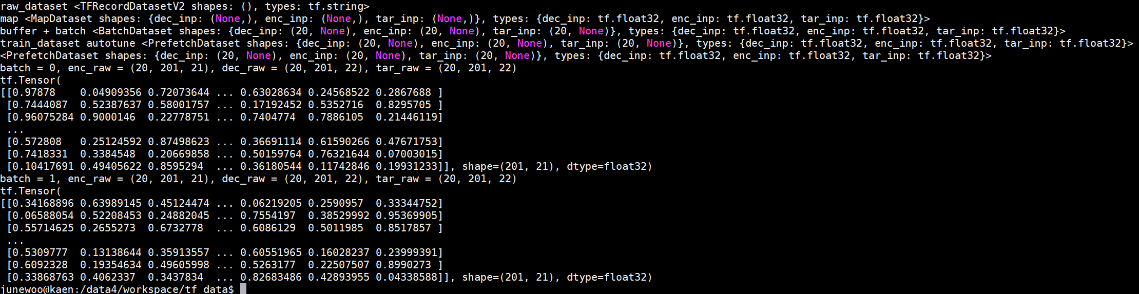
Tensorflow는 pytorch의 dataloader처럼 queue를 사용하여, 전체 데이터셋을 가져온 뒤 그것을 batch 만큼 쪼개서 하는 것이 살짝 번거롭다.


즉 이말을 다시 풀어보면, pytorch에서는 dataloader를 사용하여 여러 queue를 사용해서 batch 만큼 데이터셋을 가져온 뒤, 이것을 tensor로 바꿔서 model에 넣는 것이 수월한데 비해


Tensorflow에서는 tf.data.Dataset.from_tensor_slices 를 사용해서 전체 데이터셋을 가져오는 예제가 많다.


게다가 대용량 데이터셋을 사용하게 될 경우, 데이터셋의 총 사이즈가 3GB 정도가 넘어가면 tensorflow 는 API 관련 오류가 생기면서 data load가 안 될 때가 있다.


근 3일 정도 고생하면서 찾아본 정보들을 합쳐서, 음성 데이터셋의 stft 한 결과인 2차원 데이터셋을 tfrecord로 저장하는 방법을 소개한다.


# 전처리

음성(.wav)파일 모두에 대해, 2차원 stft를 얻었다고 가정하고 진행하겠다.

stft를 바꾸는 방법은 이 블로그 내에 있다.


import tensorflow as tf
print(tf.__version__)
import os
import librosa
from glob import glob
import numpy as np


list_inp = sorted(glob('/your/input/dataset/*/*.npz'))
list_tar = sorted(glob('/your/target/dataset/*/*.npz'))

print(len(list_inp))

위의 코드는 모든 음성 파일을 .npz 라는 numpy 형태의 data format으로 미리 저장해둔 상태이고, 이것을 glob으로 가져오는 모습이다. Seq2Seq 모델의 Encoder input인 list_inp와 Decoder input, Real value input인 list_tar의 전체를 가져온다.


# Writing Tfrecords file


def serialize_example(batch, list1, list2):
    filename = "./train_set.tfrecords"
    writer = tf.io.TFRecordWriter(filename)
    
    for i in range(batch):
        feature = {}
        feature1 = np.load(list1[i])
        feature2 = np.load(list2[i])
        print('feature1 shape {} feature2 shape {}'.format(feature1.shape, feature2.shape)) 
        feature['input'] = tf.train.Feature(float_list=tf.train.FloatList(value=feature1.flatten()))
        feature['target'] = tf.train.Feature(float_list=tf.train.FloatList(value=feature2.flatten()))
        
        features = tf.train.Features(feature=feature)
        example = tf.train.Example(features=features)
        serialized = example.SerializeToString()
        writer.write(serialized)
        print("{}th input {} target {} finished".format(i, list1[i], list2[i]))
        

serialize_example(len(list_inp), list_inp, list_tar)


먼저 저장할 tfrecords filename을 정해주고, tensorflow에서 제공해주는 TFRecordWriter로 writer를 선언한다.

for i in range(batch)는 전체 batch 사이즈만큼 반복하는 것이다. 즉 전체 데이터셋을 저장할 것이다. (나의 경우에는 총 8백만개이다.)


numpy 형태의 파일을 sorted(glob())으로 가져왔기 때문에, 현재 함수의 인자값인 list1과 list2는 파일 경로이다. 그러므로, np.load를 사용하여 feature1과 feature2에 값을 넣어준다.


그 뒤 tfrecords에 저장할 feature['name'] tf.train.Feature(float_list=tf.train.FloatList(value=feature1.flatten()))을 하여 선언해준다.


2d numpy 값을 그대로 value=feature1 를 해주면, 오류가 생긴다. 이를 찾아보게 되면, tensorflow에서의 FloatList는 1차원 값만 넣어줄 수 있기 때문이다. 그러므로, flatten()을 하여 넣어준다.


나 같은 경우 input과 target을 모두 maximum legnth를 구하고 zeropadding하여 shape을 아는 상태이지만, 만약 데이터셋이 모두 다를 경우 feature['shape'] = tf.train.Feature(int_list=tf.train.IntList(value=feature1.shape) 을 대입하여 나중에 데이터셋을 실제로 model에 넣을 때 shape을 기억하여 변환할 수 있다.


그다음 features = tf.train.Features(feature=feature)를 통해 tensorflow의 tensor로 변환해주고,

example 또한 마찬가지로 변환해준다.


serialized = example.SerializeToString() 을 통하여 binary? 로 변환해준다. 마지막으로 tf.records 파일을 write 해주는 writer.write(serialized)를 해주면 끝난다.

이것을 batch size만큼 해준다...


전체코드는 아래와 같다.


# 전체 코드

import tensorflow as tf
print(tf.__version__)
import os
import librosa
from glob import glob
import numpy as np


def serialize_example(batch, list1, list2):
    filename = "./train_set.tfrecords"
    writer = tf.io.TFRecordWriter(filename)
    
    for i in range(batch):
        feature = {}
        feature1 = np.load(list1[i])
        feature2 = np.load(list2[i])
        print('feature1 shape {} feature2 shape {}'.format(feature1.shape, feature2.shape)) 
        feature['input'] = tf.train.Feature(float_list=tf.train.FloatList(value=feature1.flatten()))
        feature['target'] = tf.train.Feature(float_list=tf.train.FloatList(value=feature2.flatten()))
        
        features = tf.train.Features(feature=feature)
        example = tf.train.Example(features=features)
        serialized = example.SerializeToString()
        writer.write(serialized)
        print("{}th input {} target {} finished".format(i, list1[i], list2[i]))


list_inp = sorted(glob('/your/input/dataset/*/*.npz'))
list_tar = sorted(glob('/your/target/dataset/*/*.npz'))

print(len(list_inp))
serialize_example(len(list_inp), list_inp, list_tar)


input, target 각각 8백만개 씩 있는데, 이것들이 과연 tfrecords를 통해 저장하였을 때의 공간적 이득과, 시간이 얼마나 걸리는지 체크해봐야겠다.


체크 해본 뒤, Tfrecord 파일을 다시 원래대로 음성 데이터 spectrogram으로 복구하는 것을 이번주내로 올릴 예정이다.

728x90

+ Recent posts